Midterm 2 Review
PH142
Spring 2019
Navigating these slides
Exam logistics
Note to Students
Material
PPDAC Applications
Bias
Probability
Chapter 9
Probablity
Sample Space
Probability Model
Probability Rules
Probability Rules
Notation
Discrete models
Continuous models
Density Curve
Sampling with Code
Sampling with Code
Chapter 10
Dependence and Independence
Multiplication Rule for Independent Events
Conditional Probability
General addition rule for any two events
Example
Example
Example
Example
Example
General multiplication rule
Bayes' Theorem
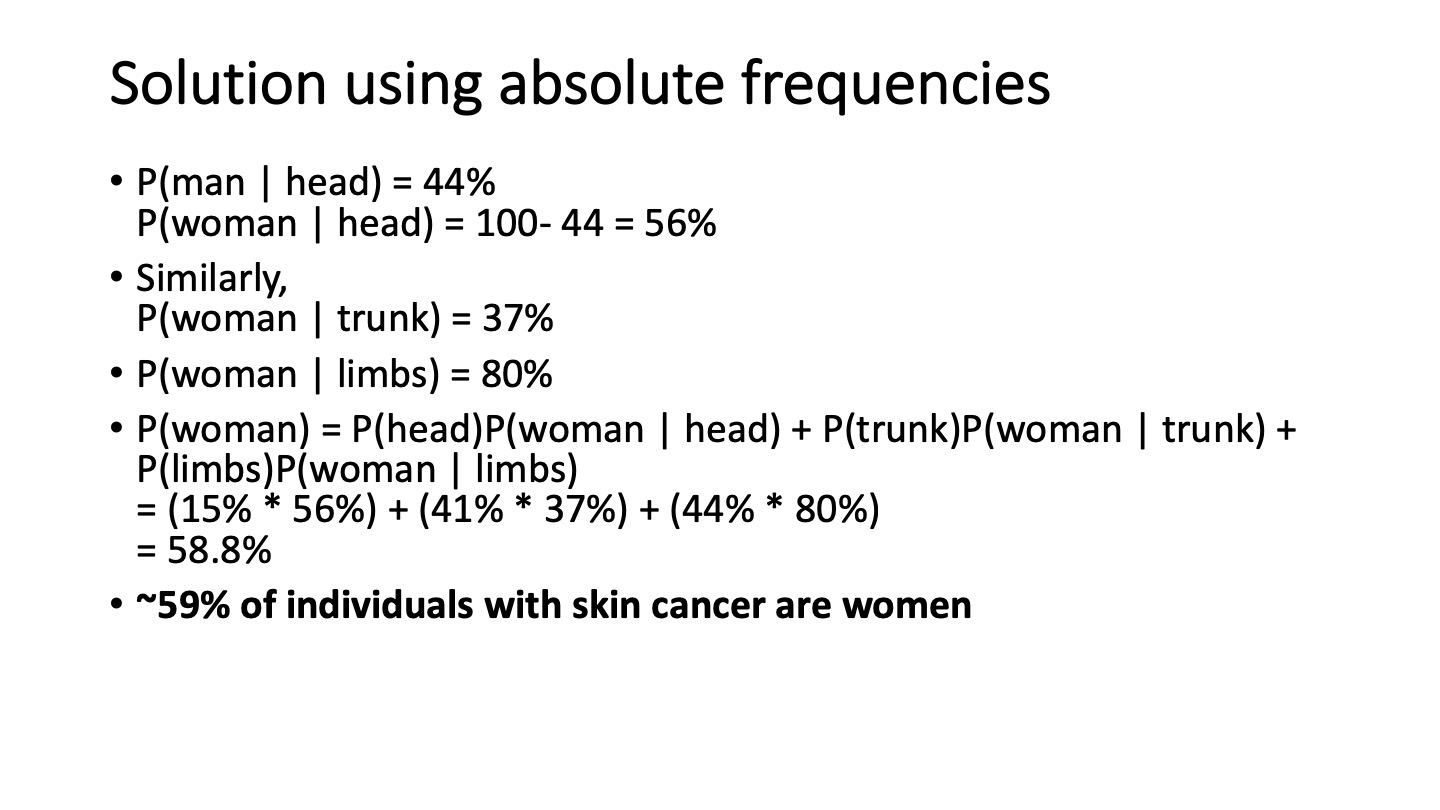
Absolute frequencies and tree diagrams
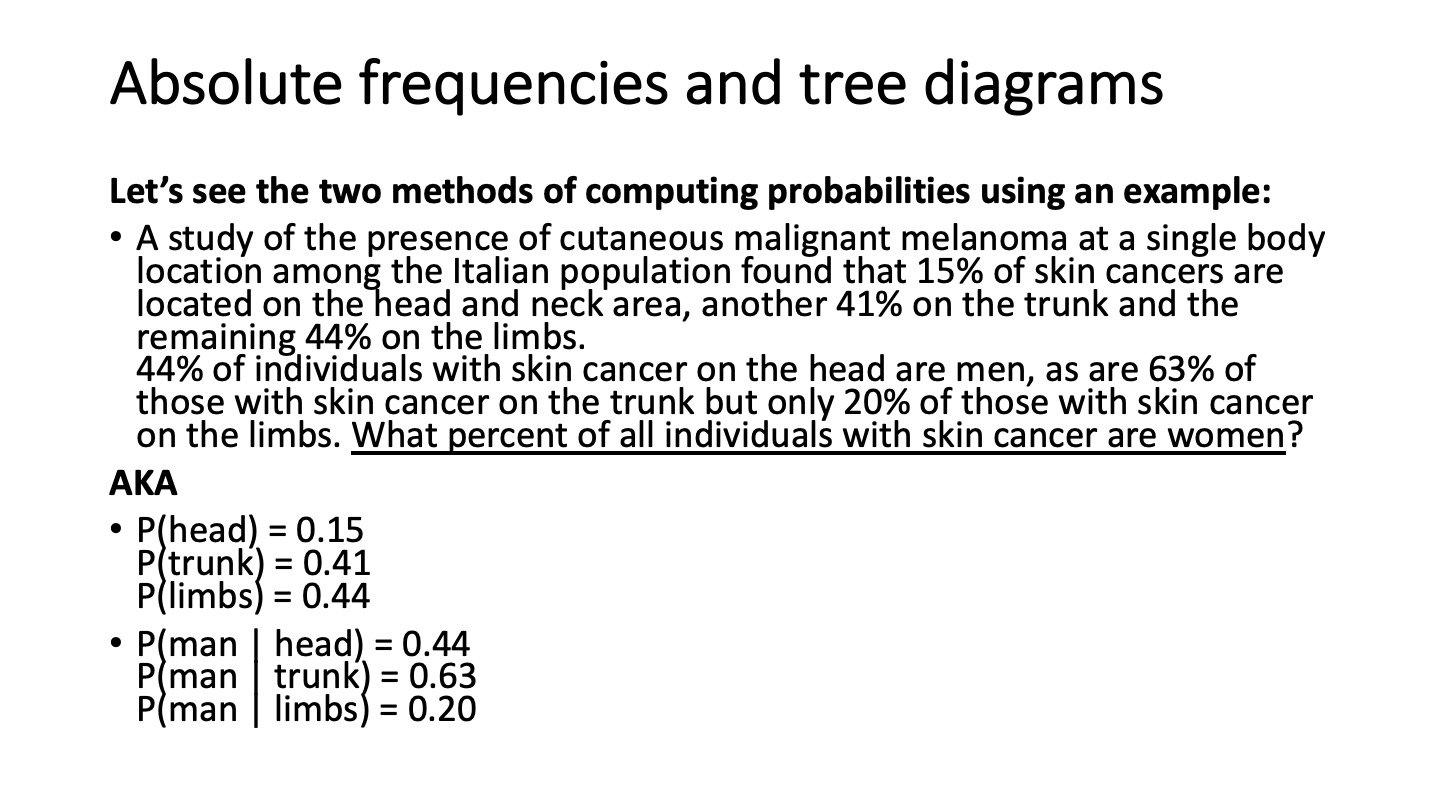
Absolute frequencies and tree diagrams
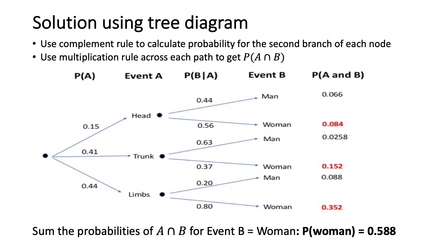
Absolute frequencies and tree diagrams
Distributions
Chapter 11: Normal Distribution

Recipe for Normal
Question
Example
Example
Chapter 12: Binomial and Poisson Distributions
Binomial
Binomial
Normal Approximation for the Binomial Distribution
- If we have a binomial distribution that satisfies the below properties, we can approximate the distribution as a normal distribution instead
- This allows us to use all the awesome properties we know about normal distributions (very convenient!)

Example
Example
Example
Example
Example
Poisson
Example
Sampling Distributions
A sampling distribution is the distribution of estimates that we have for our parameter. In our case, we either make distributions of estimates for \( \mu \) or population proportion \( p \).
Chapter 13
Here's a motivating figure from the text. After you're done looking over this section, reflect on this figure and see if you can understand it all.

Law of Large Numbers
Law of Large Numbers
Law of Large Numbers
Law of Large Numbers
Law of Large Numbers
Law of Large Numbers
Central Limit Theorem
Central Limit Theorem
Central Limit Theorem
Exploring the Population (“The Underlying Distribution”)
This is the distribution of the population salaries.

Central Limit Theorem
Central Limit Theorem
Central Limit Theorem
Sampling with n=2
ggplot(sample_means_2, aes(x=mean_salary)) +
  geom_histogram(binwidth=0.7) +
  scale_x_continuous(limits = c(0, 40))

Central Limit Theorem
Sampling with n=5
ggplot(sample_means_5, aes(x=mean_salary)) +
  geom_histogram(binwidth=0.5) +
  scale_x_continuous(limits = c(0, 40))

Central Limit Theorem
Sampling with n=30
Visually, the sample size of \( n=30 \) is the most symmetric.
ggplot(sample_means_30, aes(x=mean_salary)) +
  geom_histogram(binwidth=0.5) +
  scale_x_continuous(limits = c(0, 40))

As \( n \) gets larger, then we see the sampling distribution get less skewed and more like the normal curve.
Sampling Distribution Means and Variances
Chapter 14, 15
Hypotheses
Confidence Intervals
Confidence Intervals
Confidence Intervals
Z-testing
Z-test conditions
Step 1: Hypotheses
Step 2: Z-value calculation
Step 3: Finding the p-value
Once we have our z-value, we can find the p-value. To help find the p-value, sketch the standard Normal curve and mark on it the observed value of z. Depending on whether you are performing a one-sided test or a two-sided, this will determine in which direction you calculate the p-value/probability:
Here is a visual to illustrate the differences
#
Use pnorm() functions to calculate your p-value. Remember we are working with a Standard normal.
Step 4: Interpreting p-values
Step 4: Interpreting p-values
Example (try on your own)
Example (try on your own)
Type I and II Errors

Types I Error

Critical value

Types II Error

Power

Power
