Lab 8. From zee to tea-tests.¶

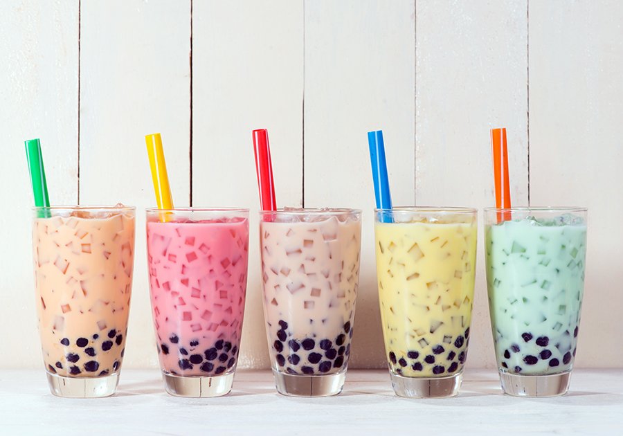
Aside: I'm a stats nerd, so I can make so many allusions to statistics when looking at a boba drink. I'll start you up on one then carry on before I get too nuts. Let the liquid part of the dessert be a sample space. Let the crystal jelly stand for Event J, and let the black pearls stand for event B. The sample space is 100%. Do we have intuition on the probabilities of Event B and Event J? Do they add up to 100%?!

Back on topic: What do you call the following beverage? Growing up, my friends and I would call it "boba". When I hang out with my family in New York, they call it "bubble tea". I always found it odd, but not too odd because occasionally "bubble tea" would appear on menus.

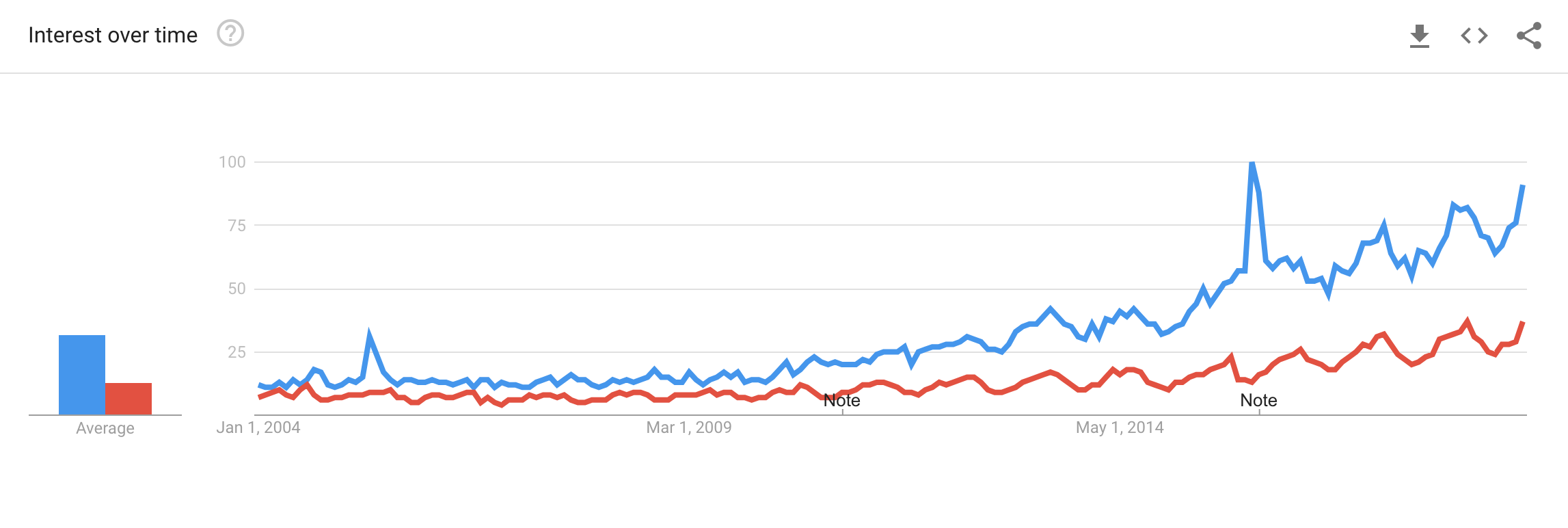
According to Google Trends, both terms have increased in search queries over time! The below plot is called a "time series plot", and we briefly mentioned time series in the first part of the class.

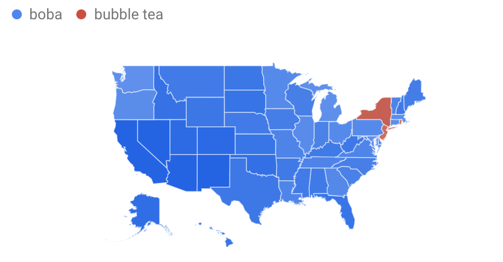
And nope, this is not a presidential election map. The blue shows states for which "boba" is the more popular term. The red shows states for which "bubble tea" is more frequented.

Testing for the mean of "boba"¶

Imagine we believed that the Google interest in "boba" was 50 points overall for all time periods. Let the data we have stands for a random sample of "boba" interest throughout the years. How can we test?

library(readr)
tapioca <- read_csv("data/multiTimeline.csv")

Parsed with column specification:
cols(
  Month = col_character(),
  boba = col_integer(),
  bubbletea = col_integer()
)

Let's preview the data, which we will consider the data to be an "independent sample"! (Even if it's not! Just bare with me, it was a fun pedagogical idea...)

head(tapioca %>% select(boba))

We are interested in the hypotheses:

$H_0: \mu=50$
$H_0: \mu \neq 50$

Can we use a z-test?¶

Before we do any test, we have to check assumptions.

Is the underlying population normal?
Do we have an independent, random sample?
Do we know the population standard deviation?

No, we can't... because we don't know #3.

Can we do something else?¶

Yes. We can estimate the population standard deviation with the sample standard deviation. A long time ago in a galaxy (the same as this one), William Goset learned the theory behind the t-distribution. Long story short, instead of doing a normal-distribution-based-hypothesis-test, we're going to do a t-distribution-based-hypothesis-test. (I put hyphens so you can tell which pieces go together...)

library(dplyr)
t.test(tapioca %>% pull(boba), alternative="two.sided", mu=50)

	One Sample t-test

data:  tapioca %>% pull(boba)
t = -11.19, df = 182, p-value < 2.2e-16
alternative hypothesis: true mean is not equal to 50
95 percent confidence interval:
 28.96766 35.27278
sample estimates:
mean of x 
 32.12022

Comparing the mean searches of "boba" and "bubble tea"¶

Assume we are interested in the mean Google interest of "boba" and "bubble tea" since 2004 (not exactly something you would do in real life since this is time series data, but it's interesting to try out). I took data from Google Trends to explore them in R.

And let's look at some statistics.

library(dplyr)
tapioca %>% summarize(avg_boba=mean(boba), sd_boba=sd(boba), avg_bt=mean(bubbletea), sd_bt=sd(bubbletea))

Attaching package: ‘dplyr’

The following objects are masked from ‘package:stats’:

    filter, lag

The following objects are masked from ‘package:base’:

    intersect, setdiff, setequal, union

head(tapioca)

Do the averages between "boba" and "bubble tea" look about the same?

I'm going to use melt() to reshape my data. Don't worry about this function.

library(reshape2)
tapioca <- melt(tapioca, id.vars="Month")

library(ggplot2)
library(RColorBrewer)
ggplot(tapioca, aes(y=value, group=variable, fill=variable)) + 
    geom_boxplot() + 
    xlab("") + 
    ggtitle("Interest in Boba and Bubble Tea on Google") +
    theme_bw() +
    scale_fill_manual(values = c("dodgerblue", "firebrick2"))

The boxplots look different front each other in different ways. Look back at your previous notes and describe the differences using statistical language. While the boxplots are indeed different, they overlap! How can we test if the means are really different from one another?

$H_0: \mu_{\text{Boba}} = \mu_{\text{Bubble tea}}$
$H_1: \mu_{\text{Boba}} \neq \mu_{\text{Bubble tea}}$

By hand¶

# * BY HAND PT. 1/
diff_in_mean <- mean(tapioca$boba) - mean(tapioca$bubbletea)
diff_in_mean

# * BY HAND PT. 2/
se <- sqrt((var(tapioca$boba) / nrow(tapioca)) + (var(tapioca$bubbletea) / nrow(tapioca)))
se

# * BY HAND PT. 3/
t <- diff_in_mean / se
t

Without knowing our degrees of freedom before going into this, we're not going to be able to calculate the p-value "by hand". In this class, you do not need to calculate the degrees of freedom for a two sample t-test. Let $df = 225.22$.

# * BY HAND PT. 4/4
2*(1-pt(t, 225.22))

Some points:

I multipled by 2 because I have a two-sided test.
I subtracted the pt() from 1 because my diff_in_mean > 0. If it was < 0, then I wouldn't subtract from 1.
There is an almost 0% chance of observing the data that we did GIVEN that the two distributions have the same mean. (Almost because there is some rounding done on the computer that we don't see.)

Using R functions (t.test and dplyr functions)¶

# * USING R FUNCTION
t.test(x=tapioca %>% pull(boba), y=tapioca %>% pull(bubbletea), alternative="two.sided")

	Welch Two Sample t-test

data:  tapioca %>% pull(boba) and tapioca %>% pull(bubbletea)
t = 11.15, df = 225.22, p-value < 2.2e-16
alternative hypothesis: true difference in means is not equal to 0
95 percent confidence interval:
 15.52518 22.19067
sample estimates:
mean of x mean of y 
 32.12022  13.26230

Treating the data as paired¶

These data, technically, can be treated as pairs since they are taken at the same time point and have to deal with the interest in the same subject matter (gooey starch balls!) The hypotheses will change now.

$H_0: D_i=0 \, \, \forall i$
$H_1: D_i \neq 0 \text{ for some } i$

head(tapioca %>% mutate(boba-bubbletea))

tapioca <- tapioca %>% mutate(d=boba-bubbletea)
t.test(tapioca %>% pull(d), alternative="two.sided")

	One Sample t-test

data:  tapioca %>% pull(d)
t = 16.966, df = 182, p-value < 2.2e-16
alternative hypothesis: true mean is not equal to 0
95 percent confidence interval:
 16.66481 21.05103
sample estimates:
mean of x 
 18.85792

Month	boba	bubbletea
2004-01	12	7
2004-02	11	8
2004-03	11	9
2004-04	13	10
2004-05	11	8
2004-06	14	7